Home > Features >

Go to QFI Archives >>

IN QUEST OF INFINITY – 22

By Prof. G. Venkataraman

---

Loving Sai Ram and greetings from Prashanti Nilayam. Last time, I made an attempt to introduce you to the world of Quantum Mechanics [QM] which, many feel, is the most important scientific development of the twentieth century. That is because QM compelled us to change entirely our approach to the world of the small. And such a change in thinking was absolutely essential to explore issues connected with the mysteries of the Universe, especially how the Universe itself came into being.

Now there are two basic aspects to Quantum Mechanics. One is the “Tool Box” aspect and the other is the Philosophical Aspect. As far the former is concerned, this dual aspect of QM is best exemplified by a remark due to a distinguished Physicist [I believe it was David Mermin] who told his students, “Shut up and calculate!”

What he is supposed to have meant is: “Students, the philosophical implications of QM are extremely subtle and we are not sure even after seventy years what exactly to make of it. If you enter that realm, you would simply get lost.

However, at the working level, QM gives a good set of working rules like grandma’s medicines. Just use those rules, crank the wheel and do calculations to get practical answers to practical questions. That can help a lot.

Leave all the worrying about the philosophical underpinnings to egg-heads who do not have to worry about getting research contracts, promotions etc! If you want to survive, just shut up and calculate!”

We do not know if the Prof actually said that to his students, but that remark attributed to him does indicate the complexities underlying QM. That there were such complexities became evident even in the early days, and in this issue, I shall offer you some glimpses of that, as also where the enquiry of those days led subsequently; all that makes a very fascinating story!

Quantum Discoveries

Now where exactly do I begin? Maybe I should start by recalling the sequence leading to the birth of QM. I narrated that story last time, but just to get going with this issue, let me do a bit of recall. Essentially four things happened, almost in an unconnected manner, but having deep connections nevertheless.

Getting back to the early days, by around 1930 or so, one had a formal scheme called QM, using which, one could, in principle, start calculating many things, like the energy levels of the hydrogen atom, for example. Earlier, one had to do this using Bohr’s rather artificial model [see QFI – 20, 21].

	A wavefunction of an electron in a hydrogen atom

Thanks to Dirac, one had a much better way of doing that calculation and getting much better results too. Of course, all this was at the non-relativistic level, but for the moment let us set that complication aside. At any rate, for the sake of record I might state that Dirac in fact wrote the relativistic equation for the electron, which proved to be another important break-through; but then, I am drifting away from what I want to say presently.

Returning to our main theme, people now began to say: “Well, this QM certainly works. True, in many cases the mathematical problems to be solved are horrendous, but then, we faced that problem in classical mechanics too. One thing must be said, however; in classical mechanics, we understood what was going on, and there were no mysterious entities, like the Uncertainty Principle and the wave function.”

The wave function Ψ introduced by Schoredinger did seem like a big puzzle. What exactly did it mean? This Ψ was supposed to be a complex quantity. But in Physics, we do not have any complex quantities, only real numbers. How then did this Ψ sneak in? It seemed so essential and yet its role was so elusive. Did it have any physical meaning at all, and could it in fact have any? Such were the questions troubling many.

The smarter ones focussed on publishing papers, ignored such issues and improved their rating with a string of papers and discoveries. As someone said, those were times when second-rate men could do first-rate work! But there were others who did worry about the philosophical implications of this new mechanics called QM. One of them was Max Born, whom we met briefly earlier.

Born’s Search for the Real

Born thought and thought about Ψ. He said, “Listen, we simply cannot have a complex quantity having a physical meaning. But one thing we do know from mathematics. If we take a complex quantity and multiply it by its complex conjugate, we get a real quantity. Should I be looking for something like that here, before searching for meaning?”

I should perhaps add a few words of explanation that would make clear the lines along which Born was trying to go. Consider a complex number like say, 2 + i3, where, if you recall from my earlier explanations, i is the square root of -1, and is an imaginary number. The number (2 + i3) is called a complex number having both a real as well as an imaginary part. The real part is 2, while the imaginary part is 3.

The complex conjugate of this complex number, denoted as (2 + i3)* has the value (2 – i3). Thus, the product (2 + i3) x (2 + i3)* = (2 + i3) x (2 –i3) = 2 ² + 3 ² = 13; and 13 is a real number. I hope that is clear. What I am driving at is that while Ψ introduced by Schroedinger might be a complex quantity, the product ΨΨ* is a real quantity and could therefore perhaps be assigned a meaning. Thus Born said to himself, “I shall not try to find a meaning for Ψ but for ΨΨ*.”

After exploring for a while, Born did succeed in finding the meaning of ΨΨ*, and that sure was a major breakthrough in the conceptual understanding of QM. Let me now try to explain what physical interpretation Born gave to ΨΨ*. By the way, the contribution of Born, monumental though it was, remained ignored for a long time, and was rewarded with the Nobel Prize only much later – thank God his contribution was finally acknowledged!

Understanding the contribution of Max Born is crucial and so let us spend some time over it. Basically, what Born said [after much reflection of course] was the following:

That is what Born said, and I realise that terse statement would not make much sense to you. So, let us go over all that a bit more slowly. First of all, when we talk of a wave amplitude, we must specify the point at which we are considering the amplitude. The meaning of this observation would become clear from a reference to Figure 1.

FIGURE 1: This figure shows a wave. Clearly, the wave has a physical extension. Marked in the figure are a few space points, P1, P2, etc. From the figure it is evident that the amplitude at these points are different. Thus, when one talks of a wave amplitude, one must also specify the space point one is considering. That is, if A is the symbol representing the amplitude of the wave, we should really talk in terms of A(r), where r denotes the space point under consideration. By the way, presently we are considering a static wave, that is a wave that does not change with time. In general, waves could change with time, like a wave on the surface of the sea for example. Such waves are called time-dependent waves and in such cases when one speaks of the amplitude, one should quantify it as A(r, t), where t denotes the time at which we are considering the wave amplitude at the point r.

From the figure above, it should be clear that when Born interprets ΨΨ* in terms of probability amplitudes, he should really be talking of ΨΨ*(r). By the way, we are considering what are called stationary quantum states, that is, states that do not change with time. That means we do not have to deal with Ψ(r, t) but only with Ψ(r); I hope that is clear.

Quantum Orbits

	The mini solar system of the Bohr atomic model

OK, now how do we take all this further? This is best done by going back to the Bohr atom model. You would recall [see QFI – 20] that Bohr visualised the atom to be something like a mini-solar system, with the electron going round in various orbits around the nucleus, which played a role similar to our Sun, as the main centre of attraction.

In the case of the hydrogen atom [which, remember is the simplest atom in Creation], there is only one electron revolving round the nucleus, and this electron has many orbits to chose from.

Of course, each orbit has its own energy, and by choosing different orbits, the electron can occupy different energy states – all this we have been through before.

Let us stay with this simple model and consider one particular instant of time. It is like taking a photograph of the hydrogen atom with such a short exposure that during the exposure, the electron has hardly moved; we would then see the electron as if it were frozen at one spot in the orbit it is moving along.

Suppose we take many such photos and superpose all of them; we would then get a picture something like in Fig. 2

FIGURE 2: This is a schematic of what we would see if an electron obeying the Bohr model were to be photographed repeatedly and all those photos were superimposed. All we would see would be a series of dots, as in (a), each dot representing the position where the electron was, when the snap was taken. If the electron were to be photographed say millions and millions of times and all these photos are once again superimposed, then in this case, we would see more or less a closed orbit as in (b). I guess you can understand why.

Let us now carry over this idea to the Schoredinger equation and all that. Here is what we do. First, we start with the Schroedinger equation for the hydrogen atom; next it is solved. When this is done, one ends up with any number of solutions. These are then indexed. [I believe the big man himself did all this]. Now how do we label these different solutions that turn up? That is simple because Schroedinger himself has told us how to.

In 3 D, electrons photographed millions of times and then superimposed would create the spheric 'shells' of the atom

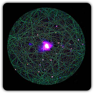
Remember what Bohr did? He labelled his solutions with integers, 1, 2, 3, etc. So his index was n, where n could take on all integer values, 1, 2, 3, ….etc. The orbits corresponding to these different values for n were what Bohr called the stationary states of the hydrogen atom. Schoredinger found that the solutions for Ψ(r) the wave-function of the hydrogen atom did require an index n [like Bohr had]; but there was also a need for another index, which was denoted by l. Thus, in the Schoredinger picture we had Ψ_n,l (r), characterising the stationary states of the hydrogen atom.

Before we proceed further, we need to know what this new index l is and what values it can take. First, the allowed values for l; suppose the index n has the value 3 say. In this particular case, l can take the values 0, 1, and 2. If similarly n were equal to 5, then l would take on the values 0, 1, 2, 3, 4, and so on. In general, l could take on the values 0, 1, 2, ….. up to (n-1). Hope that is clear.

And so we now have two indices characterising the stationary states of the hydrogen atom in the Schroedinger scheme, which means we have to deal with Ψ(r) for the (n,l) combinations: (1, 0); (2, 0) and (2,1); (3, 0), (3, 1) and (3, 2); (4, 0), (4, 1), (4, 2) and (4, 3) etc. Clear? Hope so! There is one more complication, but that we shall come to that later.

Let us now ask a simple question. “Bohr had a solar-system model. Suppose we had a 2 D hydrogen atom in the Schoredinger picture. What would ΨΨ*(r) look like for n =1? Remember, in this case, the only allowed value of l is 0. So when we talk of n = 1, we are really dealing with the case (n, l) = (1, 0). The question we are asking is, to use the language earlier used: “Suppose we take repeated snap shots of the electron in the state Ψ_{1, 0} (r), superpose it and all that. What would we get? That picture is shown in Fig. 3.

FIGURE 3: This figure is a “superposition of snapshots” when the [2 D] hydrogen atom is in the state Ψ1, 0 (r). The nucleus is in the centre and is shown as a much bigger dot than it really ought to be; this is done for the sake of clarity of seeing. We observe, as we saw earlier, a collection of dots, a cluster really as opposed to one that roughly defines an orbit. In other words, QM demolishes the notion of orbits! Instead, the electron in a particular state is spread out into a fuzzy cloud.

I hope you have digested the main message of Fig. 3. In case you feel a bit confused, imagine a fellow shooting bullets at a target, as in rifle practice. The man is aiming at the bull’s eye, but does not always hit it. However, he hits close, but occasionally misses the target by a wide margin. If the target is taken out after a time and examined, you might see something like in Fig. 4.

FIGURE 4: This is a schematic of a target shot during rifle or pistol practice. The shooter always aims at the Bull’s Eye, but misses it most of the time. The pattern of misses is what we see here. If the shooter is a good one, most of the bullets would cluster near the centre, whereas if he is a poor shooter, most of the bullets would miss by a wide margin. On the whole, this gives some idea of the probability that the shooter would hit the Bulls Eye.

OK, what Fig. 4 is supposed to do is to tell us that the schematic in Fig. 3 is a probability pattern of where we might find the electron around the nucleus, when it is in the Ψ_{1, 0} (r) state. Hope you are able to follow that. Notice that the stationary states of the atom do NOT correspond to the electron moving in well-defined orbits; rather, the electron is “spread into a kind of cloud”. Remember, this “cloud” picture comes from first solving for the wave function Ψ(r), then calculating ΨΨ*(r) for various values of r, and then plotting a dot for each value of r with a number corresponding to the value of ΨΨ*(r).

Electron orbital wave functions of hydrogen atom

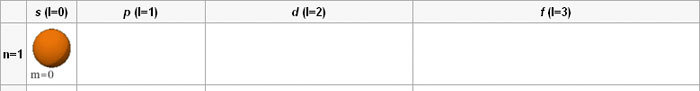
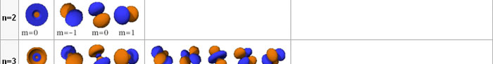
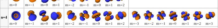
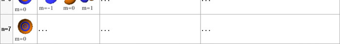
In the schematic figure shown in Fig 3, the values for ΨΨ*(r) are not shown. Instead, what is shown is a scatter of points that is representative of these numerical values. That is to say, if the probability is high, we have a high packing, while if the probability is small, we have a low packing of points. In the figure, we see that the cluster of points is congested for small values of r. That means that the probability for the electron to be near the nucleus is greater than when it is far.

That is how one must read this figure. In short, it is best to imagine the electron cloud to be something like a cotton-candy puff, of varying density! I hope you have noticed that I have stopped referring to the electron moving in an orbit and instead am talking about the probability of finding the electron at different points. This is a major paradigm shift, brought about by QM.

Quantum Density Distribution

So now the question becomes: “What kind of cotton-candy puffs would represent the stationary states of the hydrogen atom?” Well, a whole library of pictures have been produced corresponding to these various stationary states, by patient calculations of course. However, before I present them to you, there is one more detail, an important one, that I must mention.

Remember I said that two indices, n and l are needed for indexing the stationary states of the hydrogen atom in Schoredinger’s picture? It turns out that we actually need one more called m [sometimes labelled l_m ]. By the way, n and l are not just called indices but quantum numbers. Thus n is called the principal quantum number while l is called the orbital quantum number. In the same way, m is called the magnetic quantum number.

What about the restrictions on m? Just as for a given n, l was restricted to the set 0, 1, 2,…..(n-1), for a given l, the quantum number is restricted to the set l, ( l -1)….., 0, -1, -2,….. – ( l -1), - l. Thus, if l = 3 say, then m would take the values 3, 2, 1, 0, -1, -2, and -3. Given below is a sample table that shows the manner in which the various quantum numbers form a hierarchy.

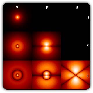
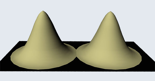
Very nice pictures have been made using software to illustrate the electron distribution associated with the various possible states indicated in the above table, but before I discuss that, there is one more point I must bring to your notice so that you are able to appreciate the pictures that I shall soon present.

FIGURE 5: Shown here is an example of a weather map. What I would like you to note are the lines drawn across the map. These lines connect points that correspond to places having the same atmospheric pressure. In the map above, we have many lines, each marked with a number. Follow the line with the number 1008. You would see it forms a loop. All the towns, villages and cities lying on this particular curve have the same pressure, measured as 1008 in some units. A line connecting points having the same pressure is called an isobar. Thus the map above is an isobaric map. Such maps are very useful for the weather man. For example, in the map above, one can see loops within loops, the smallest one carrying the number 992. This shows that there is a Low-pressure trough. And that sure means bad weather is coming to that region! What have weather maps to do with electron clouds? For that, return to the main text!

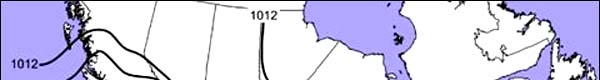
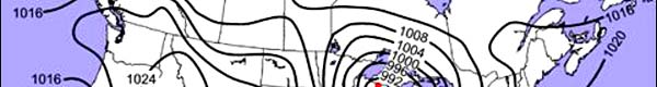
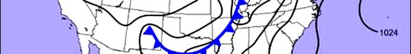
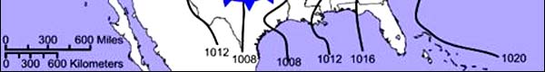
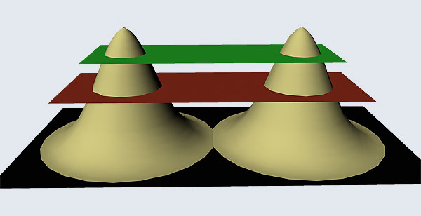
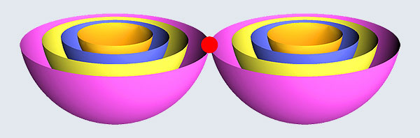
The main reason why I digressed into weather maps is draw your attention to the concept of connecting points having the same property with a continuous line. An isobar is one such line; it connects points on a weather map that have the same atmospheric pressure. Similarly, let me consider maps showing {Ψ_{n, l, m} (r) Ψ*_{n, l, m} (r)}. I am sure you understand what the quantity within the brackets { } means. It means the probability of finding the electron at the space point r, when the electron is in the state labelled by the triad of quantum numbers n, l, and m.

Suppose I now join all points that have the same value for ΨΨ*. Note the points are different; however, the quantum numbers remain the same [since we are talking of a particular electron state] and the numerical value of ΨΨ* also would be the same. So what do we expect at the end of it all? We expect to see a surface such that all points on the surface correspond to the same numerical value for ΨΨ*, for, of course, the state defined by particular values for {n, l, m}. This surface would be like the isobar I introduced to you earlier; so maybe you would now understand the significance of the digression into weather maps.

OK, with all that preamble and preparation, I guess I can now unleash some nice pictures!

FIGURE 6: Shown here are what are called atomic orbitals, corresponding to the various quantum states that the hydrogen atom can be in. The concept of atomic orbitals is explained further in a BOX that comes at the end. Don’t miss that!

There are a few important things I must draw attention to here. The first relates to the “cotton candy” aspect of the electron density distribution. What these pictures show is the expected [probability] density of electrons in the neighbourhood of the nucleus. Thus, the electron is more likely to be found in certain places than elsewhere. I hope you are able to follow that.

Electrons Have No Trajectories

Next comes the whole issue of electron trajectory. In classical mechanics, trajectories play an important role. When a bullet is fired, for example, it follows a particular trajectory. A lot of problems that students have to solve deal with such classical trajectories. In QM, the idea of trajectory disappears!

This was in a vague way realised at the time the Bohr model appeared. Bohr no doubt started with the idea that the electron perhaps moved in circular orbits, but no where in his calculations do the actual trajectories appear. Sure there are states labelled by the quantum number n, and sure, one talks of the radii of the various orbits, but no mention of actual trajectories and electrons actually going round and round in such orbits.

There was no need to; Bohr just wanted to know the energies of the levels, and the energy differences for that gave him an idea of the hydrogen atom spectrum, which after all was his goal [see QFI – 20]. And he got what he wanted without discussing actual trajectories.

The work of Schoredinger and the subsequent interpretation of Max Born showed that orbits really had no place in QM. I mean, go back to Fig. 3 which shows a lot of dots. Let us say that the electron was found at a spot corresponding to one of these dots at a particular instant. Can anyone say where the electron would go to in the next instant, from that starting spot? No one can! In fact, a little closer examination shows that the idea of trajectories has no meaning at all in QM! And do you know why? It is all because of Heisenberg’s Uncertainty Principle [see QFI – 21]!

To define [an ideal] trajectory, one must know precisely where the electron was from one instant to the next. In classical mechanics, if one knows where the electron was at time t₁ say, and also knew precisely the momentum of the electron at time t₁, then one could, using the equations of classical mechanics, calculate precisely where the electron would be at some other later time t₂.

In QM, on the other hand, if at time t₁ we know precisely where the electron was, then we do NOT know precisely what the momentum was at that same instant – that is the Uncertainty Principle for you! In short, the whole concept of a definite trajectory is lost. The “cotton candy” aspect introduces a fuzziness! All that is due to the probabilistic nature inherent in quantum mechanics; and thanks to that probabilistic nature, first called attention to by Max Born while figuring what Schroedinger’s Ψ meant, erupted a famous controversy or debate I should perhaps say.

This, by the way, was no ordinary debate, but one between two great giants – Einstein on one side and Bohr on the other. The debate was long and protracted, and ran over many years. But out of that came many ideas and many issues, some of which still remain, making QM one of the strangest aspects of Nature.

Squeezing the Space within Iron

Just to give you an idea of how strange things can be, let me draw your attention to the following strange fact. Suppose you consider iron. The iron atom has 26 electrons around its nucleus. The size of the nucleus would be roughly 10 ^-11 cm, quite small. If we think in terms of the Bohr picture, we would have a solar system with many orbits, each containing some electrons; in all, there would be 26 electrons of course, as shown schematically in the figure below. The largest orbit would have a size of about a few time 10 ^-8 cm.

FIGURE 7: This figure is a schematic of the iron atom, as one would visualise it in the Bohr model. The basic idea of this figure is to convey that at the centre is a tiny, tiny atomic nucleus with a diameter around 10 -11 cm, while around this miniscule nucleus are circulating 26 electrons that are even tinier [each electron may be around 10 -16 cm!]. What it all means is that the atom is mostly empty space. But the miracle is that when we put a lot of such “empty spaces” together to form a piece of iron and try to squeeze it, we find it hard! Strange is it not? Well that is all due to the mysteries of QM. Thanks God for that, for it were not for that, we all would have fallen through the earth long ago!

What the above figure shows is that by and large the iron atom is empty, rather like our solar system. But hold on for a minute. Suppose we pack a lot of iron atoms together, we would get a piece of iron, may be as big as a nail [it would have to be a large number of atoms, something like 10 ²² !]. So we have this piece of iron which we find to be very solid, though every atom is supposed to be practically empty. Strange, is it not?

But wait! Try holding the iron piece and squeezing it. You just would not be able to; this we know from experience. But why is the iron not squeezing? After all, every atom is almost empty; and when we squeeze, all we are trying to do is to move the atoms close to each other; with so much empty space available, it should be very easy to squeeze the iron piece, since every atom should be able to literally move through other atoms.

Yet, squeezing iron is so tough! Odd, is it not? Well, that is where QM pulls its magic. You may not believe it, but it is the “cotton candy” nature of the electrons as opposed to the orbit picture that I tried to sell above, that makes atoms so hard to press against each other. Remember way back I told you about stars called White Dwarfs and Neutron Stars? Their exotic properties all have to do with the strange way electrons behave, thanks to QM.

In short, it all goes right down to the probabilistic nature of QM. Einstein was shocked by the probabilistic message QM was trying to give. Suddenly, determinism was out of Physics, and it seemed as if God was playing dice! How on earth could God do that? No wonder the poor Prof. lost sleep! All that story in the next issue!! Till then, all the best.

P.S. PLEASE DO NOT MISS THE BOX WHICH SUPPLEMENTS THE ABOVE WITH SOME INTERESTING INFORMATION ABOUT ELECTRONS IN ATOMS.

	When one studies carefully the “cotton-candy” patterns that the electron in the hydrogen atom could adopt in the various allowed quantum states, one is filled with wonder. I mean all this serves a great purpose, that God obviously knew in advance, which is why, I think, He endowed the simple hydrogen atom with such richness, via QM that is. What exactly do I mean? To understand, please study carefully what follows. Let us start with a hypothetical one-dimensional atom with a nucleus and one electron. In this case, one of the many possibilities for the electron to position itself with respect to the nucleus is shown in FIGURE (a) below. FIGURE (a): In this figure, we have a double-bell shaped probability distribution curve, centred around x=0 where the nucleus is supposed to be. On the x-axis are marked points 1, 2, 3, 4, 5, …etc. The probability of finding the electron at these points is given by the values P1, P2, P3, etc., that can be read off the electron density distribution curve. I hope this is clear. If we try to make a “map” of points with same values, we would get a plot as in Fig. (b). FIGURE (b): Let us now consider a two-dimensional atom. There is a nucleus and one electron, that can move in 2 D. In this case, the Electron Density Probability Distribution curve becomes a surface with two sheets as shown in Fig. (c). Basically, this shape is obtained by rotating each of the two independent curves of Fig. (a); I am sure you can easily follow that. FIGURE (c): Next, let us try to locate points on the plane where the electron distribution would have equal values; this would be like drawing isobars on the weather map. To do this, we first slice the two mountains with horizontal planes as shown in Fig. (d). FIGURE (d): I am sure you can see that each such plane would cut the “mountain” along a circle. If all these circles are plotted together, we would get what is shown in Fig. (e). We have a set of concentric circles, each corresponding to one particular value for the electron density – just like in the isobar map. FIGURE (e): Let us now move to 3 D, which is the realistic case. In this case, if we tried to depict a “mountain plot” we would need four dimensions! I am sure you can follow that – for a 1 D atom we needed two dimensions to show the mountain plot. For a 2 D atom our mountain required three dimensions for portrayal. In the same manner, for a 3 D atom would have a four dimensional mountain. Living as we do in 3 D, we cannot depict such a mountain- sorry about that! However, we can certainly do something that is the equivalent of drawing circles as in Fig. (e). And that something is shown in Fig. (f). FIGURE (f): We have here instead of nested circles as in Fig. (e), a set of nested spheres. For convenience of visualisation, these spheres have been cut across, so that you can see the different spheres, one within the other, just as we had one circle within another in the previous figure. OK, all this is fine but what is big deal about God being clever? That is what I am coming to. You see, if you consider the immense richness in the “cotton candy” patterns that even the simple hydrogen pattern provides, then you sure must wonder: “Why all this?” Well, God did it all with a grand purpose! And you know what that purpose is? Just look at the molecules in Nature; there are millions and millions of them, starting with the simple molecules like the hydrogen molecule itself (H2), the water (H2O), on to an amazing number of organic molecules that include kerosene, petrol, and so on – just millions of them. And when we enter the biological world, there are millions more, all amazing molecules, from the zillions of proteins to the DNA itself. Each of these has the hydrogen atom. How on earth is the hydrogen atom able to find a place for itself almost everywhere? That is all due to the diverse “cotton-candy” patterns that the hydrogen atom can choose from. It is to make room for such diversity that God apparently, and with much forethought, made the atom into a quantum entity, thus granting the potentiality of incredible diversity! By the way, these cotton-candy patterns as I call them have a scientific name; they are called atomic orbitals, a name very familiar to chemists. It is thanks to the richness of the atomic orbitals, that Nature is able to accommodate so many diverse and wonderful molecules. In turn, these molecules provide such richness and diversity to both the inanimate and the animate worlds. And by the way, the “cotton candy” also prevents us from falling through the surface of the earth on which all of us walk! God sure is amazing, is He not? Next time you have Swami’s Darshan, try to see the enormous Glory of the Divine behind His Beautiful and Enchanting smile. He might pretend not to know many things, including your name, but don’t get fooled by all that! Take care!!

Dear reader, how do you like this series? Please share your impressions about this article by writing to h2h@radiosai.org mentioning your name and country. Thank you for your time.

Previous Articles In The Same Series
Part - 01	Part - 02	Part - 03	Part - 04
Part - 05	Part - 06	Part - 07	Part - 08
Part - 09	Part - 10	Part - 11	Part - 12
Part - 13	Part - 14	Part - 15	Part - 16
Part - 17	Part - 18	Part - 19	Part - 20
Part - 21

---